Using the Subtotal Function to Sum Filtered Data in Excel

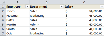
Filtering data using the Auto Filter feature is very useful. However, when using the Sum function to add up values of an applied filter, the function adds both the visible and hidden cells. Therefore, the solution is to use the Subtotal function, which only calculates the visible cells in a range.

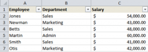
1. Display workbook in Excel containing data to be filtered.
2. Click anywhere in the data set. Click Home from the Ribbon. Click the Sort & Filter drop down from the Editing group. Click Filter. Filter drop downs display in column headings.
   
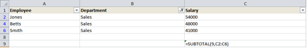
3. Apply filter on data.
4. Click below the data to sum.
5. Enter the Subtotal formula to sum the filtered data.
   Syntax to sum filtered data using the Subtotal formula:

   =Subtotal(function number, data range)

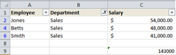
   The function number to sum filtered data is 9. Using the example in the above screen shot, the formula would be defined as follows:

   =Subtotal(9,c2:c6)
   

   

6. There are additional function numbers that can be used to subtotal filtered data. The complete table is shown below with the function number and assigned function: